Design tool
Design your own view-dependent surface
Pick up to four viewing directions and an image for each. Press Optimize to run the optimizer from the paper, then download the result as a printable mesh. The settings below are the arguments of grad_descent().
It runs in your browser. We ported the code from Python to JavaScript for this page. There is also a full-page version of the tool.
Each image is turned to face its camera, so it looks upright from that view. The Python code does not do this.
Pick views and pictures, then press Optimize.
loss per view height steps bars split rays doubled
Optimizer settings (grad_descent arguments)
After step 300 the bars are not split any further. The Python code keeps splitting them every 100 steps.
In short
We make 3D-printed surfaces that show a different picture depending on where you look from. The surface is a grid of coloured bars of different heights. From any direction, taller bars hide parts of the bars behind them, so each viewer sees a different mix of colours.
Such a surface is hard to design by hand, so we optimize it. We use a differentiable renderer for coloured heightfields. It reduces each camera ray to a 1D problem with a closed-form colour, so gradients are cheap to compute. The optimizer adjusts heights and colours until each view matches its target image. The result is printed directly on a full-colour PolyJet printer, with no lenses or coatings.
Section 3
A differentiable renderer for heightfields
A heightfield is a matrix of bar heights H and a matrix of bar colours C. It is viewed by orthographic cameras, each given by a viewing direction. This is a good model because the surfaces are shallow. For every camera i there is a desired image Di, and the renderer produces the actual image Ii.
Each pixel is a ray. In the code, the pixels lie on a grid over the surface, at its mean height, and each ray is traced back along the camera direction.
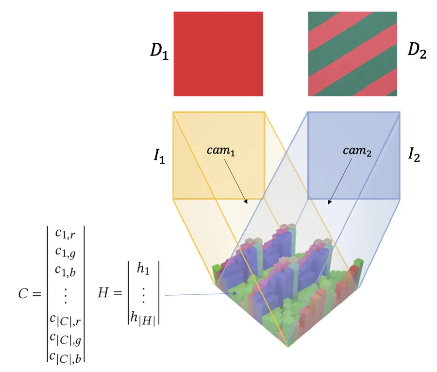
Slicing the heightfield
A ray can only hit the bars directly below its path. So we project the ray onto the ground plane, list the bars it crosses in order, and measure how far it travels through each one. This gives a 2D slice: a row of bars with heights hi, colours ci and widths wi, and a 2D ray that enters it at height oy.
The code: find_intersections, find_ids_and_lengths, get_2D_ray
rendering.py. pixel and cam come from the figure above.# traced back from z = 1, as in grad_descent.py
origin = pixel - 20 * cam
ids, widths, ray = rendering.get_2D_ray_info(origin, cam, 8)
print("bars crossed (row, col):", [(int(a), int(b)) for a, b in ids])
print("widths:", np.round(widths, 3))
print("o_y:", round(float(ray.origin.y), 3))
Rendering a single pixel in closed form
For each bar, trace a line back from its far top corner, parallel to the ray, to the line x = 0. It meets that line at height
yi = hi − (dy / dx) · Wi, Wi = w0 + … + wi (1)
where (dx, dy) is the direction of the 2D ray, which points down. A ray entering at height oy passes over bar i when oy > yi. A tall bar can hide the bars behind it, so we take a running maximum y′i = max(y0, …, yi). With the step function g, the colour of the ray is a telescoping sum:
color(p) = c0 + Σi g(oy − y′i) · (ci+1 − ci)
Each bar the ray passes over moves the colour on to the next bar. The sum ends at the first bar that blocks the ray, or at the last bar if none does.
The two strips on the right show what all parallel rays see from this side and from the other side. The same bars show different colours from each side. “Show gradients” draws purple arrows that show how each height should move to bring the pixel closer to a target colour you pick.
The code: Eq. 1, the running maximum, and the colour sum
rendering.py. H and COL are the heights and colours from the slicing figure. ids, widths and ray come from the cell above.width_sums = rendering.get_width_sums(widths)
thetas = rendering.get_backtraced_boundaries(H, ray, width_sums, ids) # Eq. 1
mono = rendering.monotonize_boundary_points(thetas) # running maximum
color = rendering.render_ray_given_boundaries(ray, mono, COL, ids, heaviside_fn="tan")
print("y_i :", np.round(thetas.numpy(), 3))
print("monotonic:", np.round(mono.numpy(), 3))
print("o_y :", round(float(ray.origin.y), 3))
print("pixel colour (RGB):", np.round(color.numpy(), 3))
ray is the slice from the cell above.Rendering all pixels, and repeating units
A camera image is made of many such rays. The slices depend only on the camera and the bar grid, not on the heights, so the code computes them once (process_rays) and reuses them at every step. For repeated patterns, the heights of a smaller unit are optimized and tiled across the surface. In the code, the heights repeat 2×2, while every bar has its own colour.
render_camera.n = 16 origins = [np.array([(i + .5) / n, (k + .5) / n, 1.0]) - 20 * cam for i in range(n) for k in range(n)] packs = [rendering.process_rays(origins, cam, 8)] image = rendering.render_camera(H, COL, packs, 1, num_repeats=1, heaviside_fn="tan")[0]
Section 4
Objective function
We minimize the pixel-wise mean squared error between the rendered and desired images of all cameras. With m×m images:
minH,C 1/(m² |CAM|) · Σi Σx,y ( Di(x,y) − forward(cami, H, C)(x,y) )²
The loss values on this page are this error, per view.
Smooth Heaviside approximations
The step function g has zero slope almost everywhere, so the heights would get no gradient. We replace it with a smooth approximation λ(x, k), where k sets the amount of smoothing. In our tests, tanh worked best, so it is the default. The forward pass still uses the exact step, so the rendered image stays exact. Only the backward pass uses the smooth version.
| approximation | λ(x, k) |
|---|---|
| circle | ½ + ½ · x / (x² + k²)½ |
| circle distance | Bern(½ + ½ · x / (x² + k²)½) |
| erfc | ½ + ½ erf(kx) |
| tanh | ½ + ½ tanh(kx) |
| log | Bern(½ + ½ tanh(kx)) |
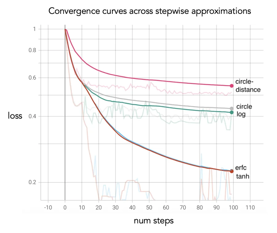
happrox.py: the forward pass of every approximation is the exact step.x = torch.tensor([-1.0, -0.1, 0.0, 0.1, 1.0])
for name, fn in [("tanh", happrox.heavi_tanh_fn), ("erfc", happrox.heavi_erfc_fn), ("circle", happrox.heavi_circ_fn)]:
print(f"{name:6s} forward:", fn(x, 0.1))
The code: HeaviTanh (forward and backward)
Regularization
Two extra terms keep the surface printable. A barrier loss keeps every height between hmin and hmax. A neighbour loss penalizes height differences between adjacent bars, which avoids thin spikes and deep gaps:
barrier = −Σi log(hmax − hi) − Σi log(hi − hmin), neighbour = Σi Σj ∈ N(i) |hi − hj|
Regularization costs some accuracy (Table 1), but it is needed for surfaces that survive printing. The original code (v1.0) uses hmin = 0.1, hmax = 1.5, and weights 0.02 (barrier) and 0.5 (neighbour). The updated code (v2.0) uses hmax = 1.0. Its neighbour loss also compares bars across the edges of the repeating unit, which avoids spikes along the seams.
| camera 1 | camera 2 | none | barrier | smoothing | both |
|---|---|---|---|---|---|
| black | white | 0.066 | 0.092 | 0.087 | 0.136 |
| black | random | 0.086 | 0.105 | 0.127 | 0.133 |
| black | stripes | 0.156 | 0.162 | 0.168 | 0.169 |
| random | stripes | 0.198 | 0.249 | 0.209 | 0.203 |
| random | random | 0.116 | 0.131 | 0.113 | 0.124 |
opt.py on the heights from the slicing figure, with the v1.0 height range.print("barrier :", round(float(opt.barrier_fn(H, min_val=0.1, max_val=1.5)), 4))
print("neighbour:", round(float(opt.neighbor_fn(H)), 4), " v2.0:", round(float(opt.neighbor_fn_wrap(H)), 4))
spiky = H.clone()
spiky[3, 4] = 1.45 # one tall spike
print("with a spike:", round(float(opt.barrier_fn(spiky, 0.1, 1.5)), 4), round(float(opt.neighbor_fn(spiky)), 4), round(float(opt.neighbor_fn_wrap(spiky)), 4))
Section 5
Optimization
The optimizer is Adam on the MSE loss, with three additions (Table 3 of the paper):
- Coarse to fine. Every 100 steps, each bar is split into 2×2 smaller bars. The surface starts with 8×8 bars and ends with 32×32. This improves the result.
- Alternating block coordinate descent. Heights and colours are updated in turns, not together. This works much better.
- Simulated annealing. Random changes to the heights and colours at the start help avoid poor local optima. This step is optional. Without it, the pattern is more uniform.
After optimizing, the target images are projected back onto the surface from their cameras. This adds detail finer than the bars. Each point is coloured from the cameras that see it, weighted by how directly they see it. To try it, press “2 · Project” in the design tool. This also trims the surface to a thin base, and the download contains the printable mesh.
| step | setting | where |
|---|---|---|
| initial surface | uniform heights 0.5, white colours; height unit 4×4 tiled 2×2 (8×8 bars) | optimize_surface.py |
| length | num_epochs = 295, i.e. 294 gradient steps (the design tool runs 600 by default) | optimize_surface.py |
| simulated annealing | 50 steps before gradient descent, T = 3 cooled ×0.99 per step, perturbations up to ±0.025 | simannealing.py |
| coarse to fine | bars split 2×2 at steps 100 and 200 (8×8 → 16×16 → 32×32); rays per view doubled 5 steps earlier (16² → 32² → 64²) | grad_descent.py |
| block coordinate descent | repeating 50-step pattern: 10 colour steps, 10 height steps, 20 colour steps, 10 height steps | grad_descent.py |
| optimizer | AdamW; learning rate 0.05 for colours, 0.03 for heights | grad_descent.py |
| camera rays | start on a plane at the current mean surface height, re-centred every 10 steps | grad_descent.py |
| projection | surface sliced thin (shortest bar 0.05 tall); desired images projected onto the visible segments of the bars, blended by how directly each camera sees them; closed textured mesh (.obj, .mtl, .png) | reproject.py |
| loss | MSE + 0.02 · barrier(0.1, 1.0) + 1.0 · neighbour (every bar against its four neighbours, wrapping around the repeating unit, averaged over bars); smooth step: tanh with k = 0.1 | grad_descent.py |
The code: the schedule in grad_descent.py
The code: the projection in reproject.py
The code: sim_annealing
| camera 1 | camera 2 | none | coarse to fine | coordinate descent | all three |
|---|---|---|---|---|---|
| black | white | 0.136 | 0.067 | 0.107 | 0.011 |
| random | random | 0.124 | 0.099 | 0.108 | 0.093 |
| black | random | 0.133 | 0.108 | 0.094 | 0.051 |
| black | stripes | 0.169 | 0.124 | 0.141 | 0.037 |
| random | stripes | 0.203 | 0.205 | 0.180 | 0.057 |
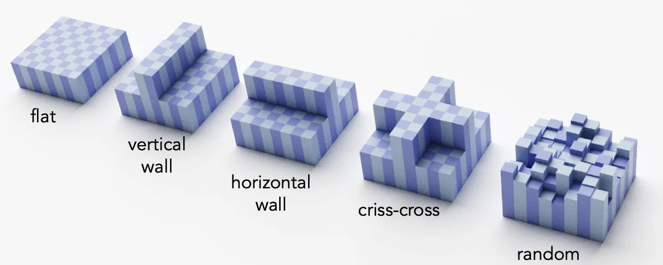
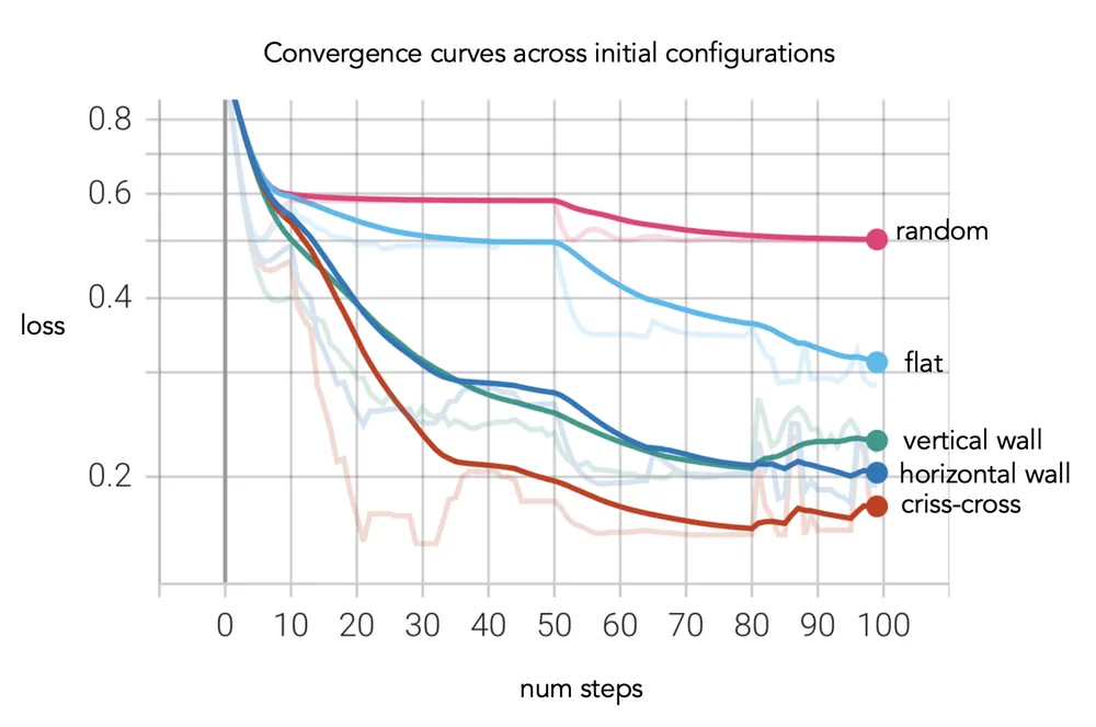
The paper also compares different starting surfaces (flat, walls, cross, random). The code starts from a flat surface.
Sections 6–8
Fabrication and results
For the paper, we turned the heights and colours into a coloured mesh in Blender and printed it on a Stratasys J55 PolyJet printer. The updated code builds the mesh in Python. Test prints showed that 300 dpi prints cleanly, which sets the smallest bar width. For surfaces under 1 cm wide, a clear top layer protects the thin bars. This layer bends light, which lowers the effective viewing angle.
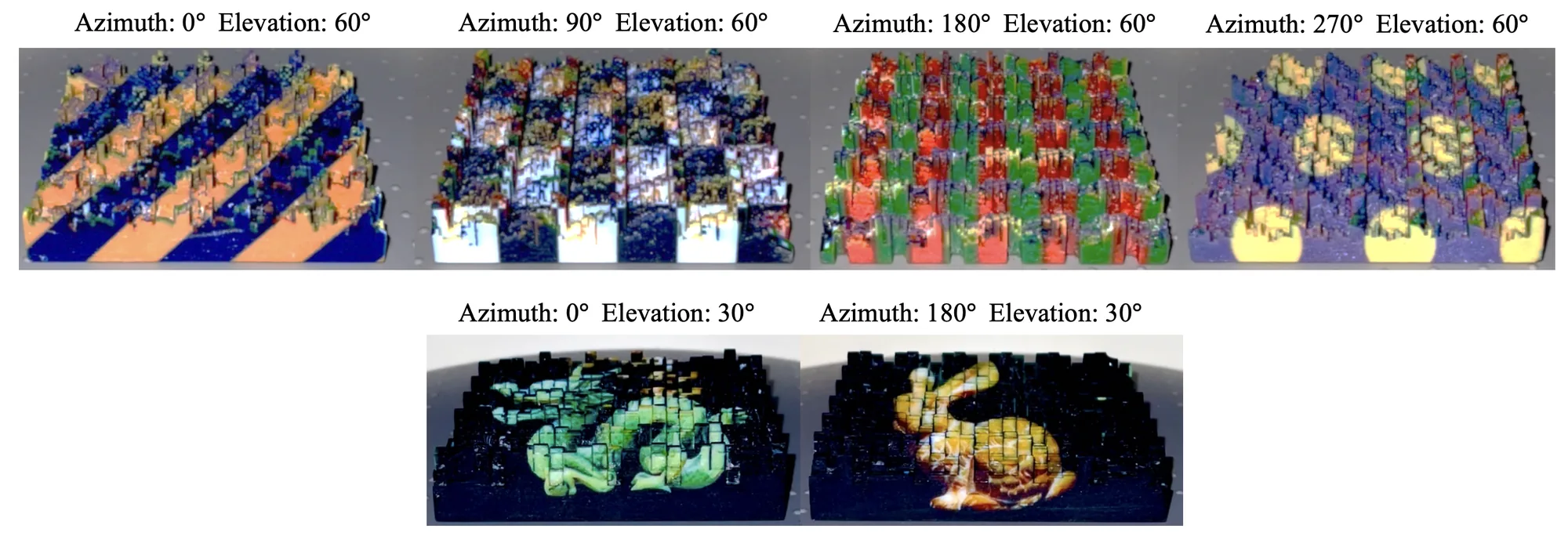
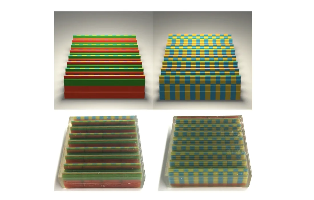
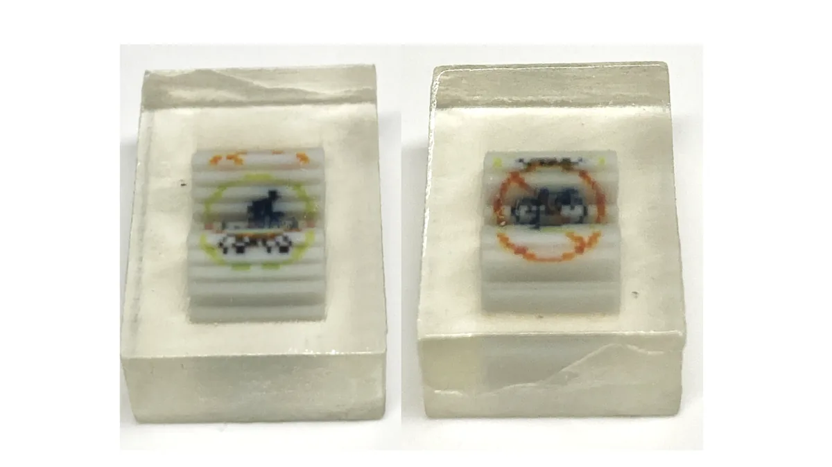
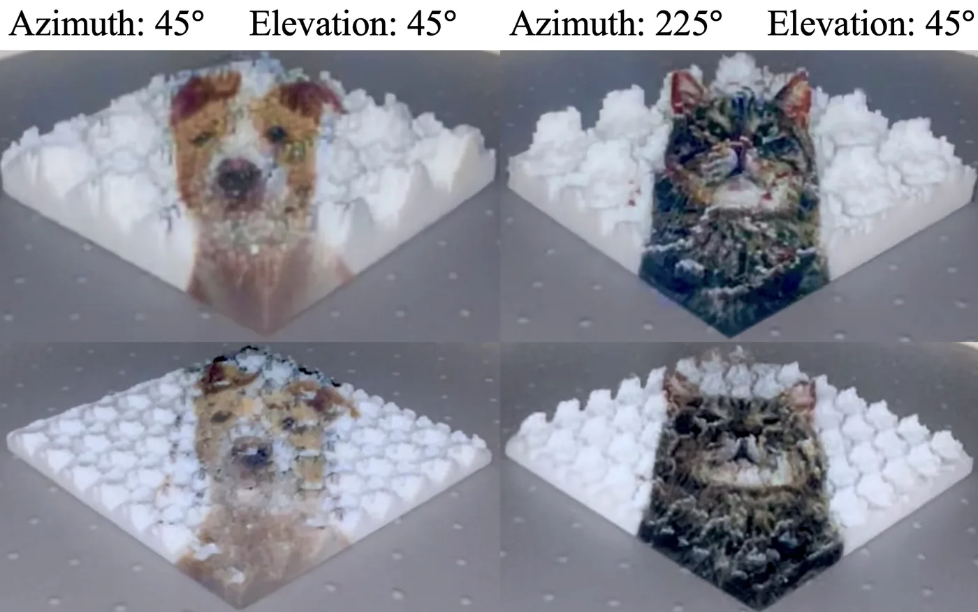
Optimization results
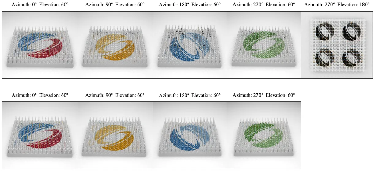
With the PyTorch code, an optimization takes 30 minutes to 2 hours. Five views work less well than four. Two views work well when they differ by more than about 40° in elevation or 60° in azimuth.
Limitations
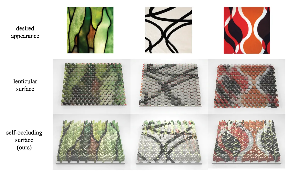
The method works for up to five views in simulation and four in print. Unlike lenticular prints, quality depends a lot on the angles between the cameras. Lighting and self-shadowing are not modelled. Future work could correct for them by adjusting the colours. On the other hand, the method reaches high resolution, can share colours between views, and uses bright colours, without the dark walls or lens arrays of earlier methods.
Citation
@inproceedings{Perroni-Scharf:2023:CPS,
  author    = "Maxine Perroni-Scharf and Szymon Rusinkiewicz",
  title     = "Constructing Printable Surfaces with View-Dependent Appearance",
  booktitle = "Proc. SIGGRAPH",
  year      = "2023",
  month     = aug
}
We would like to thank Baffour Osei and the Princeton Robotics Lab for their assistance during this project.